We frequently hear a word manifold uttered by researchers in conferences. Often it is accompanied by a picture of a curvy surface, sometimes resembling the image of an old manuscript. I felt uncomfortable that there must be a formal definition of a manifold and I don’t know it. Without understanding the fundamentals the attempts to understand the things build on top of them is inefficient. So I spend quite some time reading a section from my math book on multivariable calculus that led to the definition of a manifold. The formal definition is this:

A set M with a defined on it finite or countable atlas, that satisfies the condition of separability, is called a (smooth) manifold.

Here is a short explanation, which you can skip. Set M represents all points of an arbitraty surface, not necessarily tied to any coordinate system. We can define an injective image from a subset of M into a set of points in $\mathbb{R}^n$ , called a map. It is rarely possible to define a single map that will cover the entire set M and which is easy to work with. That’s why several maps are required. The set of maps that cover M (with certain additional restrictions) is called an atlas. The analogy is a globe, for which the atlas consists of two maps, one of the western hemisphere and another of the eastern hemisphere.

However, when reading a deep learning book, section 5.11.3 Manifold Learning, I discovered that the word manifold in machine learning isn’t used with the mathematical rigor like above. There manifold is described as just a surface (a set of connected points) in a space, which dimension (degrees of freedom) is smaller than that of the space it resides. For example, a curve in a 2D plane. Locally it has one degree of freedom (DOF) only, by moving along the tangent line at a point. Generally the dimensionality (number of dimensions) in one point can be different from the dimensionality in another point. As the example in the text goes, imagine a digit 8 drawn on a plane. Everywhere except the intersection point it has one DOF, while in the intersection point is has two DOFs.

The central idea of manifold learning is that the real data, such as images or speech, lies on a low-dimensional manifold inside a high-dimensional space. The simple experiment is this. Create a random generator of a $NxN$ matrix, restricting its values to integers in range $[0, 255]$ . Generate as many matrices as you wish, and I doubt you’ll get at least one case that looks like a real image. The probability of getting a real image is infinitely small. We can say that among all possible points in space $\mathbb{R}^n$ , real images occupy a tiny portion. This isn’t enough yet to say that those points are on a manifold, we have to show that they are connected to each other. Formally it means one had to show that there exist the first and higher-order derivatives in every point. Of course we won’t do this. Instead we conduct a second experiment, described in the same deep learning book, section 14.6 Learning Manufolds with Autoencoders, and the resulting Figure 14.6:

png

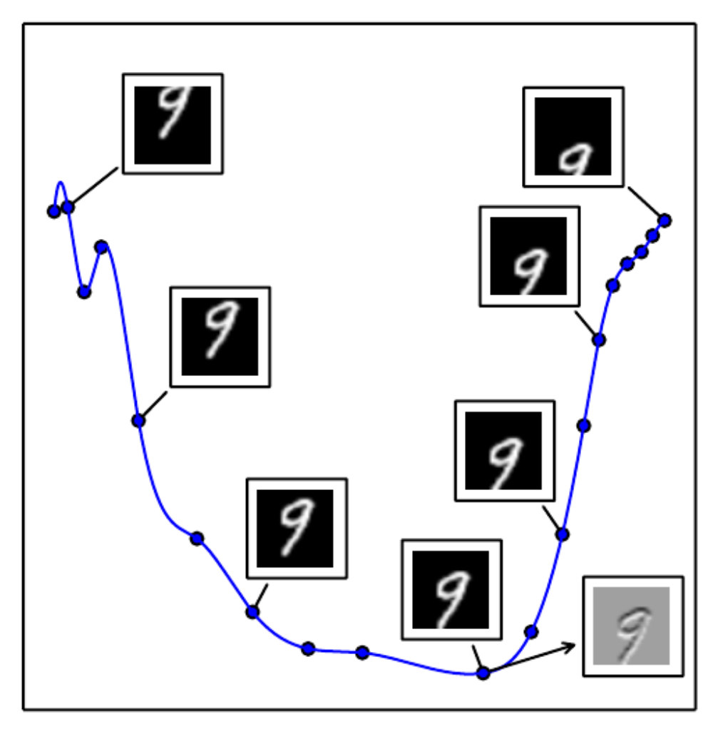
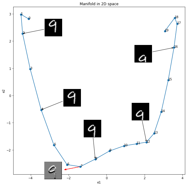
Each point in this figure represents a version of one image of 9 from MNIST dataset, translated down several pixels. We see that we can fit quite a simple curve into these points and think of it as a manifold. To make this visualization, PCA was used to project 784D points (this is what you get when you flatten 28 * 28 MNIST image) onto a 2D plane. To better understand how this figure was created, let’s try to replicate this result ourselves. And it should help to understand better what manifolds are.

Define imports

import numpy as np
%matplotlib inline
import matplotlib.pyplot as plt
from mpl_toolkits.axes_grid1 import ImageGrid
from matplotlib.offsetbox import (TextArea, DrawingArea, OffsetImage,
                                  AnnotationBbox)
plt.rcParams["figure.figsize"] = (4, 4)
from tensorflow.contrib.learn.python.learn.datasets.mnist import read_data_sets

Define plotting functions

def plim(img):
    plt.imshow(img[:,:,::-1].astype(np.uint8), interpolation='none')

def plim_g(img):
    plt.imshow(img, cmap="gray", interpolation='none')

Load MNIST dataset

d = read_data_sets("./", one_hot=False)

Extracting ./train-images-idx3-ubyte.gz
Extracting ./train-labels-idx1-ubyte.gz
Extracting ./t10k-images-idx3-ubyte.gz
Extracting ./t10k-labels-idx1-ubyte.gz

Choose the image of a digit to work with

idx = 8
img = np.reshape(d.train.images[idx], (28, 28))
plim_g(img)

png

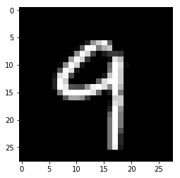
It is not exactly the same 9 as in the book, but close enough

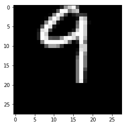
Translate vertically to a starting position

r = np.zeros((28, 28))
r[:28-6] = img[6:]
plim_g(r)

png

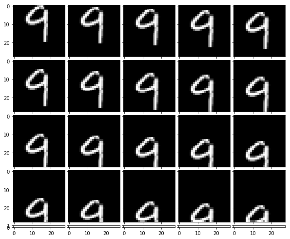
Create a set of images X, obtained by a downward translation 1 pixel at a time

Each row of X contains the coordinates of an image in some orthonormal basis

n = 20
X = np.zeros((n, 784))
X[0] = r.reshape(-1)

for i in range(n - 1):
    r[1:] = r[0:27]
    r[0] = 0
    X[i + 1] = r.reshape(-1)

Display the resulting set

fig = plt.figure(1, (10., 10.))
k = np.ceil(np.sqrt(n)).astype(int)
grid = ImageGrid(fig, 111,
                 nrows_ncols=(k, k),
                 axes_pad=0.1)

for i in range(n):
    grid[i].imshow(X[i].reshape(28, 28), cmap="gray")

png

Use PCA to project points from X onto a 2D space

The shape of X will change from [n, 784] to [n, 2]

# normalize data
Xnorm = X - np.mean(X, axis=0)
# Now we could calculate a sample covariance matrix as
# Sx = np.dot(Xnorm.T, Xnorm) / (Xnorm.shape[0] - 1)
# for unbiased estimate or ignore subtraction of 1 and simply do
# Sx = np.dot(Xnorm.T, Xnorm) / Xnorm.shape[0]
# The latter is easier from a computational point of view, 
# because we can use a fast SVD instead of a slow numpy eigenvalue decomposition np.linalg.eig

U, S, V = np.linalg.svd(Xnorm)
# returned V here is actually a V.T, 
# rows of V are eigenvectors of Xnorm.T * X

print("The first seven largest singular values", S[:7])
# Two largest singular values are of interest
print("The first maximum singular value", S[0])
print("The second maximum singular value", S[1])

('The first seven largest singular values', array([ 13.44979553,   9.24751861,   8.07277752,   7.88310738,
         7.25618232,   7.00486526,   5.59828879]))
('The first maximum singular value', 13.449795530222909)
('The second maximum singular value', 9.2475186118727013)

# keep only two eigenvectors corresponding to the two largest singular values
v2 = V[[0, 1], :]
print(v2.shape)

(2, 784)

# Project normalized data onto a 2D space spanned by those two eigenvectors
X2d = np.dot(Xnorm, v2.T)
print(X2d.shape)

(20, 2)

# approximate a derivative in one of the points (point number 7 is chosen)
diff = (X[6] - X[8]) / 2
img_diff = diff.reshape((28, 28))
# project a derivative vector onto the 2D space
diff2d = np.dot(diff, v2.T)

Plot the resulting manifold

fig, ax = plt.subplots(figsize=(10, 10))
ax.plot(X2d[:, 0], X2d[:, 1], marker='.', markersize='12')
ax.set_xlabel("e1")
ax.set_ylabel("e2")
ax.set_title("Manifold in 2D space")
for i in range(n):
    ax.annotate('%s' % i, xy=(X2d[i, 0], X2d[i, 1]), textcoords='data')
    
for i, offset in zip([2, 4, 8, 12, 16], [(100, 20), (100, 40), (-10, 100), (-20, 100), (-100, -20)]):
    im = OffsetImage(X[i, :].reshape((28, 28)), zoom=2, cmap="gray")
    im.image.axes = ax

    ab = AnnotationBbox(im, (X2d[i, 0], X2d[i, 1]),
                        xybox=offset,
                        xycoords='data',
                        boxcoords="offset points",
                        pad=0,
                        arrowprops=dict(arrowstyle="->"))

    ax.add_artist(ab)

# add the tangent vector 
ax.arrow(X2d[7, 0], X2d[7, 1], diff2d[0], diff2d[1], head_width=0.05, head_length=0.1, color='red')

# add the derivative image
if 1:
    im = OffsetImage(img_diff, zoom=2, cmap="gray")
    im.image.axes = ax

    ab = AnnotationBbox(im, (X2d[7, 0], X2d[7, 1]),
                        xybox=diff2d * 120,
                        xycoords='data',
                        boxcoords="offset points",
                        pad=0)

    ax.add_artist(ab)

png

If you are interested, you can dowload the jupyter notebook.

Summary

Manifold is a connected region, locally low-dimensional, that resides in a high-dimensional space. Real data lies on a low-dimensional manifold. It is a goal of machine learning to capture the representation of the manifold.

References

Deep Learning, Ian Goodfellow and Yoshua Bengio and Aaron Courville, MIT Press, http://www.deeplearningbook.org, 2016
Канатников А.Н., Крищенко А.П., Четвериков В.Н. Дифференциальное исчисление функций многих переменных. Москва: Издательство МГТУ им. Н.Э. Баумана, 2000.